K-Means Clustering
Overview
What is K-Means Clustering?
Why and where would we need K-Means Clustering?
How can we create K-Means Clusters?
What is our business usecase?
What business value can we extract from the clusters?
Why K-Means clustering isn’t (always) the answer?
How can we do it better?
K-Means Clustering
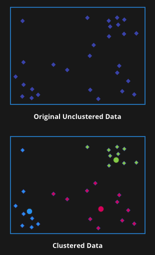
An unsupervised machine learning clustering algorithm
Data is clustered based on feature similarity
Unsupervised: Data is unlabeled, groups are unknown
Find similar groups, glean insights
Dataset may be very large and highly dimensional
Why would we need Clustering?
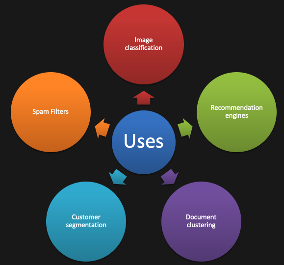
Main usecases:
A large unstructured dataset is to be clustered
without any instructionsNo prior information on how many groups we
might need to divide our data into
How can we create Clusters?
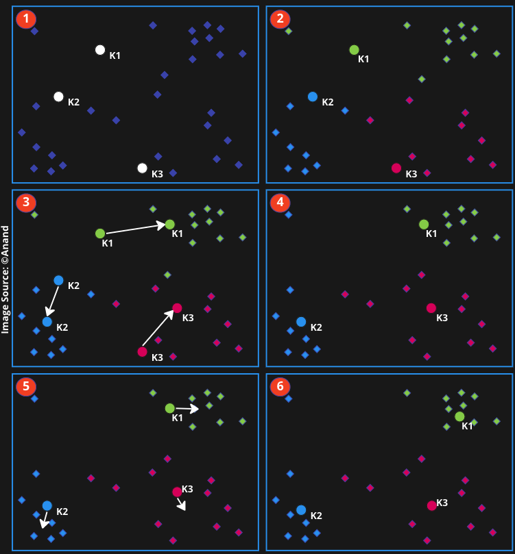
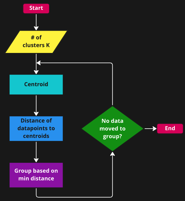
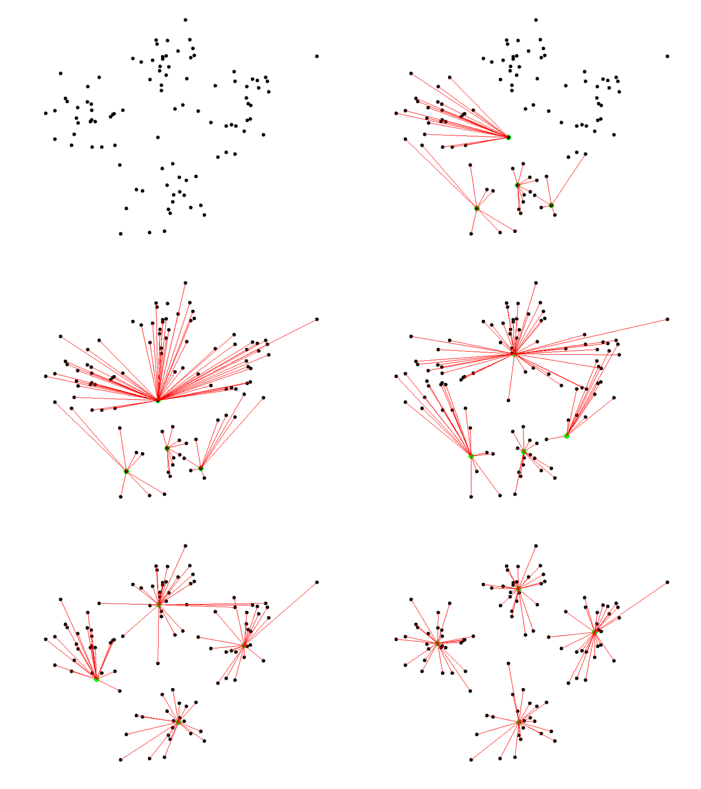

The Math behind K-Means Algorithm
- K-Means runs in an unsupervised environment and hence it measures the quality of the formed clusters by finding the variations within each cluster.
The goal will be to minimize this intra-cluster variation (also called WCSS)
\[ WCSS = \sum_{i = 1}^{k}\sum_{x ∈ C_i}|x-μ_i|^2 \]
Where, K is the # of disjoint cluster \(C_i\), x is a data point in the cluster \(C_i\), \(μ_i\) is the mean of the data points in the cluster \(C_i\).
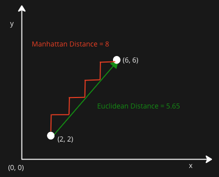
K-means calculates proximity between data points
and centroids to place the data in appropriate cluster.Euclidean distance
\[ D_{euc}(x, y) = \sqrt{\sum_{i = 1}^{n}{(x_i - y_i)^2}} \]
- Manhattan distance
\[ D_{man}(x, y) = \sum_{i = 1}^{n}|(x_i - y_i)| \]
Our Business usecase
Customer Segmentation
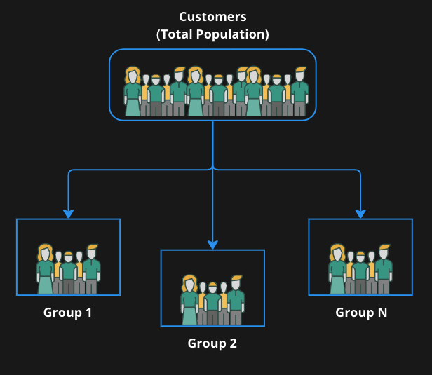
Dividing customers into number of focused groups that are as dissimilar as possible across groups, but as similar as possible within each group in specific ways with shared buying characteristics that is relevant to marketing
The chosen attributes will play a key role in deciding the groups.
Algorithm is based around analyzing what we call RFM - customer recency, frequency, and monetary values
Our Business usecase
The Dataset
The data set contains the transactions from a UK-based online retail store between 01/12/2009 and 09/12/2011.
| Attribute | Type | Description |
|---|---|---|
| Invoice | Nominal | A 6-digit unique transaction #. If starts with c, indicates a cancellation. |
| CustomerID | Numeric | A 5-digit unique customer Id. |
| StockCode | Nominal | A 5-digit code uniquely assigned to each distinct product. |
| Quantity | Numeric | The quantities of each product (item) per transaction. |
| InvoiceDate | Numeric | The day and time when a transaction was generated. |
| Price | Numeric | Product price per unit in sterling (£). |
| Country | Nominal | The name of the country where a customer resides. |
| Description | Nominal | Product name. |
| Invoice | StockCode | Description | Quantity | InvoiceDate | Price | CustomerID | Country |
|---|---|---|---|---|---|---|---|
| 489434 | 85048 | 15CM CHRISTMAS GLASS BALL 20 LIGHTS | 12 | 2009-12-01 07:45:00 | 6.95 | 13085 | United Kingdom |
| 489434 | 79323P | PINK CHERRY LIGHTS | 12 | 2009-12-01 07:45:00 | 6.75 | 13085 | United Kingdom |
| 489434 | 79323W | WHITE CHERRY LIGHTS | 12 | 2009-12-01 07:45:00 | 6.75 | 13085 | United Kingdom |
| 489434 | 22041 | RECORD FRAME 7" SINGLE SIZE | 48 | 2009-12-01 07:45:00 | 2.10 | 13085 | United Kingdom |
| 489434 | 21232 | STRAWBERRY CERAMIC TRINKET BOX | 24 | 2009-12-01 07:45:00 | 1.25 | 13085 | United Kingdom |
| 489434 | 22064 | PINK DOUGHNUT TRINKET POT | 24 | 2009-12-01 07:45:00 | 1.65 | 13085 | United Kingdom |
There are 525461 records in the dataset
107927 Customer Ids are missing (only 417534 customers are identifiable)
Our Business usecase
Data Visualization
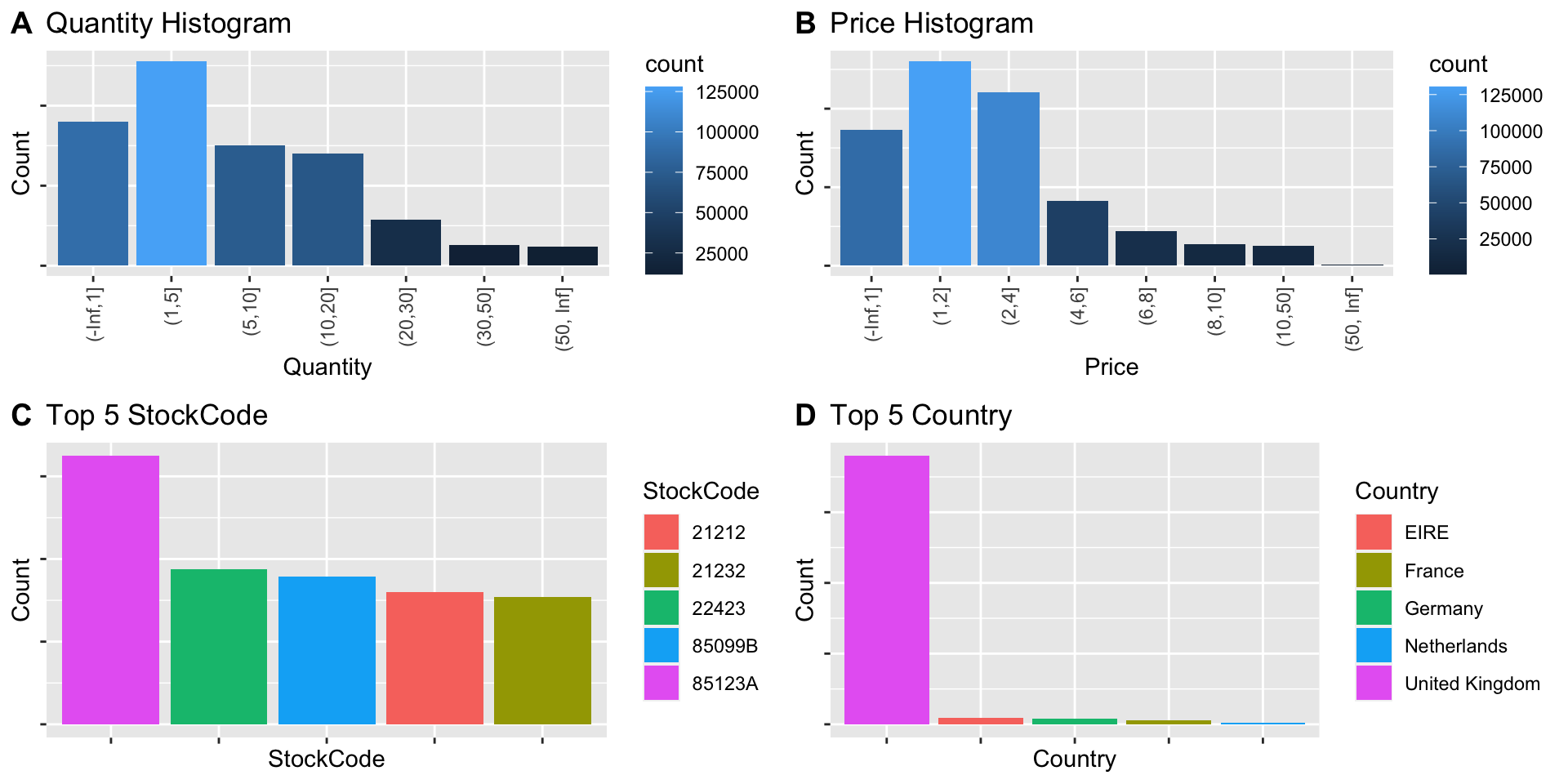
The Quantity is heavily skewed right and most of the transactions involved a quantity in the range of 1 to 5
The unit Price is also skewed right and most of the items have unit price between 1 and 4
The item with StockCode 85123A was sold most
Most of the customers belong to United Kingdom
Our Business usecase
Data Preparation
- Remove missing values
2. Select only required attributes - CustomerID,
Invoice, Quantity, InvoiceDate and Price
3. Create a new attribute Amount
- Group by customer id and count invoices
- Create a new attribute LastSeen
data$LastSeen =as.integer(difftime(max(data$InvoiceDate),
  data$InvoiceDate, units = "days"))
#Group by customer id and take min of LastSeen
customer_lastseen <-  as.data.frame(data %>% group_by(CustomerID)
%>% summarise(LastSeen = min(LastSeen)))- Merge the above data frames to get unique customer and their total amount,
frequency of visit to the store and the LastSeen shopping in the store

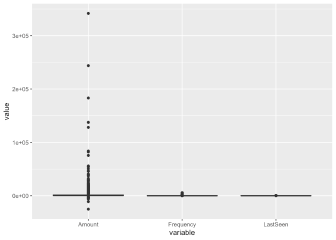
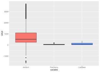
# create detect outlier function
detect_outlier <- function(x) {
    # calculate first quantile
    Quantile1 <- quantile(x, probs=.25)
    # calculate third quantile
    Quantile3 <- quantile(x, probs=.75)
    # calculate inter quartile range
    IQR = Quantile3-Quantile1
    # return true or false
    x > Quantile3 + (IQR*1.5) | x < Quantile1 - (IQR*1.5)
}
# create remove outlier function
remove_outlier <- function(dataframe,
                            columns=names(dataframe)) {
    # for loop to traverse in columns vector
    for (col in columns) {
        # remove observation if it satisfies outlier function
        dataframe <- dataframe[!detect_outlier(dataframe[[col]]), ]
    }
    return(dataframe)
}

# detect_outlier(customer$Amount)
customer <- remove_outlier(customer, c('Amount','Frequency','LastSeen'))
Our Business usecase
Target Dataset
| Attribute | Type | Description |
|---|---|---|
| CustomerID | Numeric | Customer number. A 5-digit integral number uniquely assigned to each customer. |
| Amount | Numeric | Total Amount spent by each unique customer |
| Frequency | Numeric | Number of times customer made purchases bases on their invoice. |
| LastSeen | Numeric | Days elapsed since the customer was last seen shopping. |
| Mean | Min | Q1 | Median | Q3 | Max | |
|---|---|---|---|---|---|---|
| Amount | 776.5 | -1598.7 | 241.5 | 515.1 | 1091.4 | 3685.1 |
| Frequency | 48.15 | 1 | 15.0 | 34.0 | 70.0 | 183.0 |
| LastSeen | 101.8 | 0 | 23.0 | 62.0 | 163.0 | 373.0 |
Our Business usecase
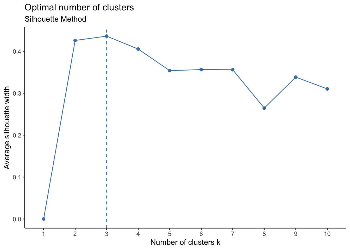
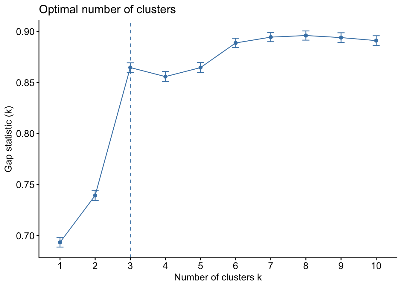
Statistical Modeling: Optimal # of Clusters
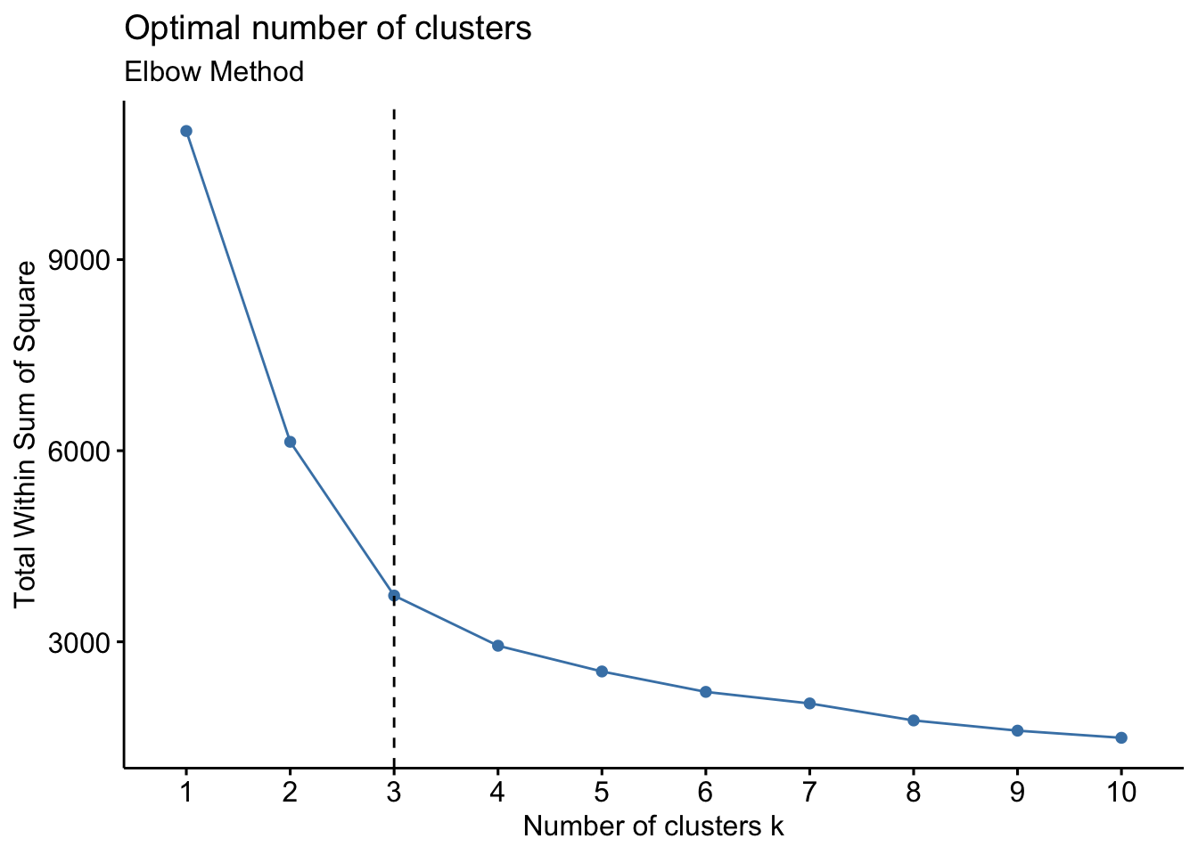
The reliability and the performance of a clustering algorithm is directly affected by the initial choice of the number of clusters (K)
fviz_nbclust(customer, kmeans, method = "wss")
  + geom_vline(xintercept = 3, linetype = 2)
  + labs(subtitle = "Elbow Method")
- Calculates values of cost with changing K
The larger number of clusters implies the data points are closer to the centroid
The point where this distortion declines the most is the elbow point
Our Business usecase
Statistical Modeling: The K-Means Model
K-Means model with K = 3
# Compute k-means with k = 3
set.seed(123)
k = 3
m1.kmean <- customer_scaled %>% kmeans(k, iter.max = 20, nstart = 25)
#nstart: Runs multiple initial configurations and returns the best one.

#Add Clusters to the original dataframe
customer$Cluster <- as.factor(m1.kmean$cluster)
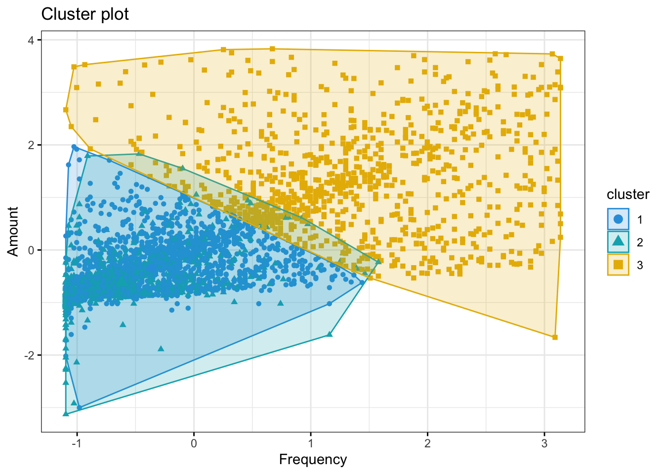
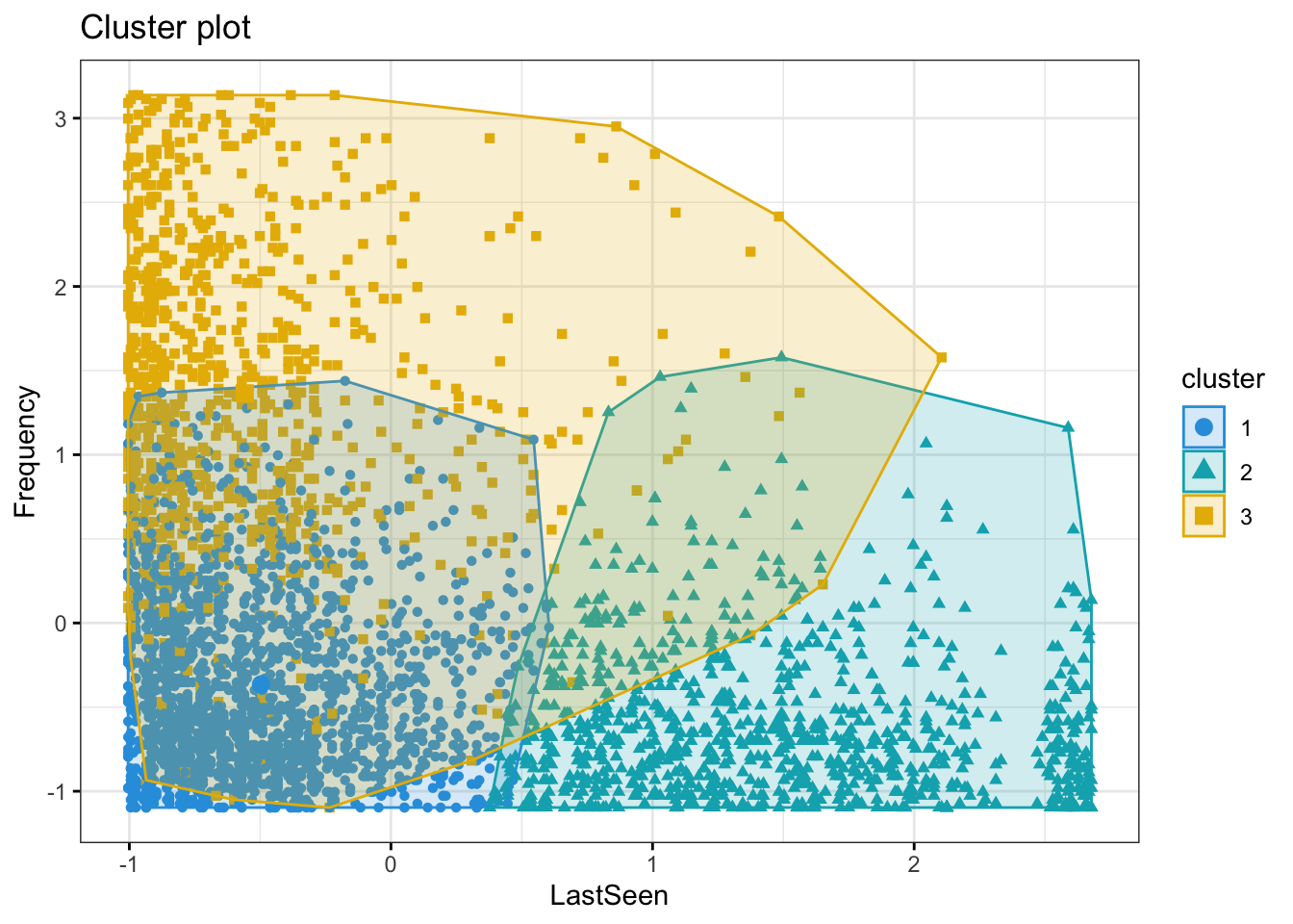
The model results in 3 clusters as was decided and the clusters are formed with sizes 1807, 953, 914.
The Business Value?
Results and Analysis
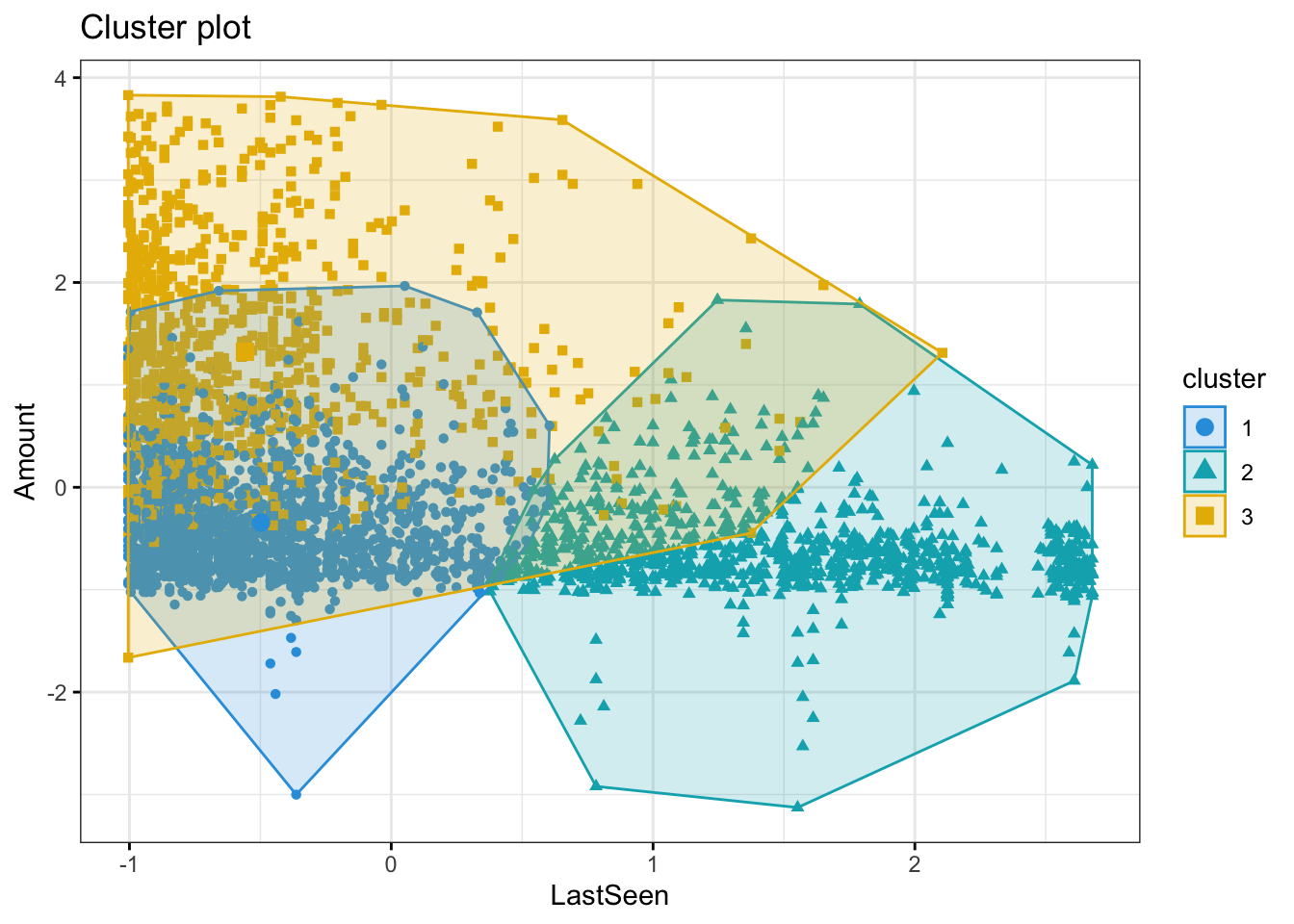
The clusters 1 and 3 are seen in the store often. Cluster 3 customers are spending more whenever they visit. Cluster 2 not seen recently so spend less
The Cluster 3 are more frequently buying and hence spending more. Cluster 1 and 2 are almost having similar trends in terms of number of purchases and amount spent
The Cluster 1 and 3 are seen buying often and whenever they are seen buying, they make lot of purchases
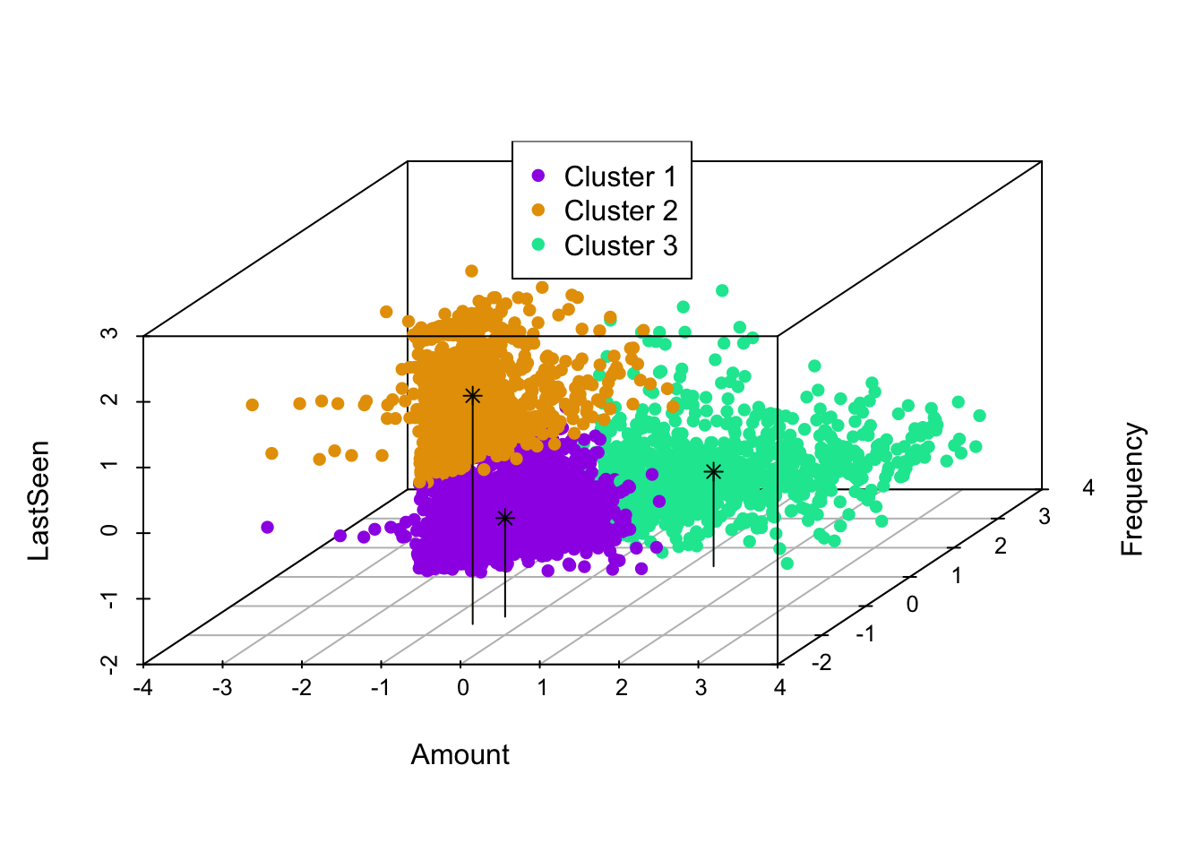
The customers in cluster 3 are seen shopping often, they spend more,
and they purchase frequentlyCustomers in cluster 2 are of concern. They do not visit the website
often but spend almost like cluster 1 and purchase as frequently as cluster 1.
So, we can either target cluster 1 to make them buy when they visit store
(since they are visiting often but buying less) or make cluster 2 visit often
as they are buying more when they visit but visiting less.
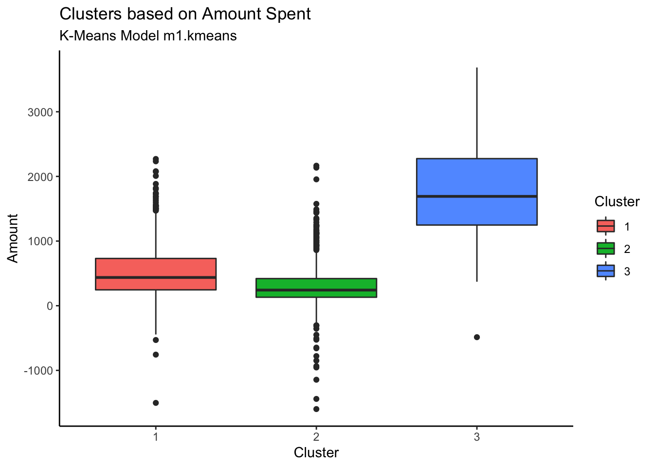
Customers in Cluster# 3 are spending more whereas cluster 2 customers are spending the least
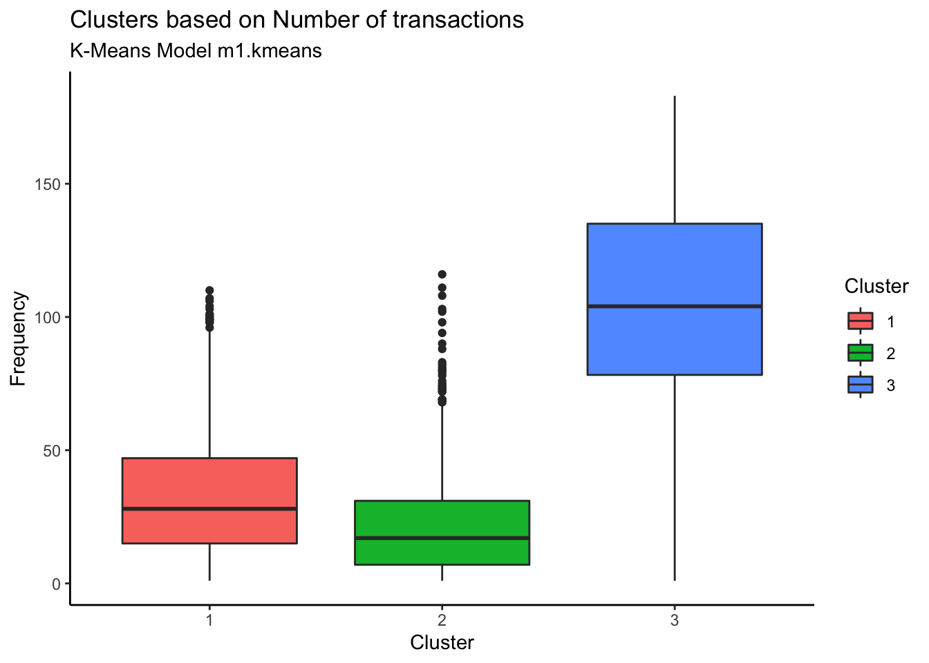
Customers in Cluster# 3 are most frequent customers indicating that the frequent customers spend the most
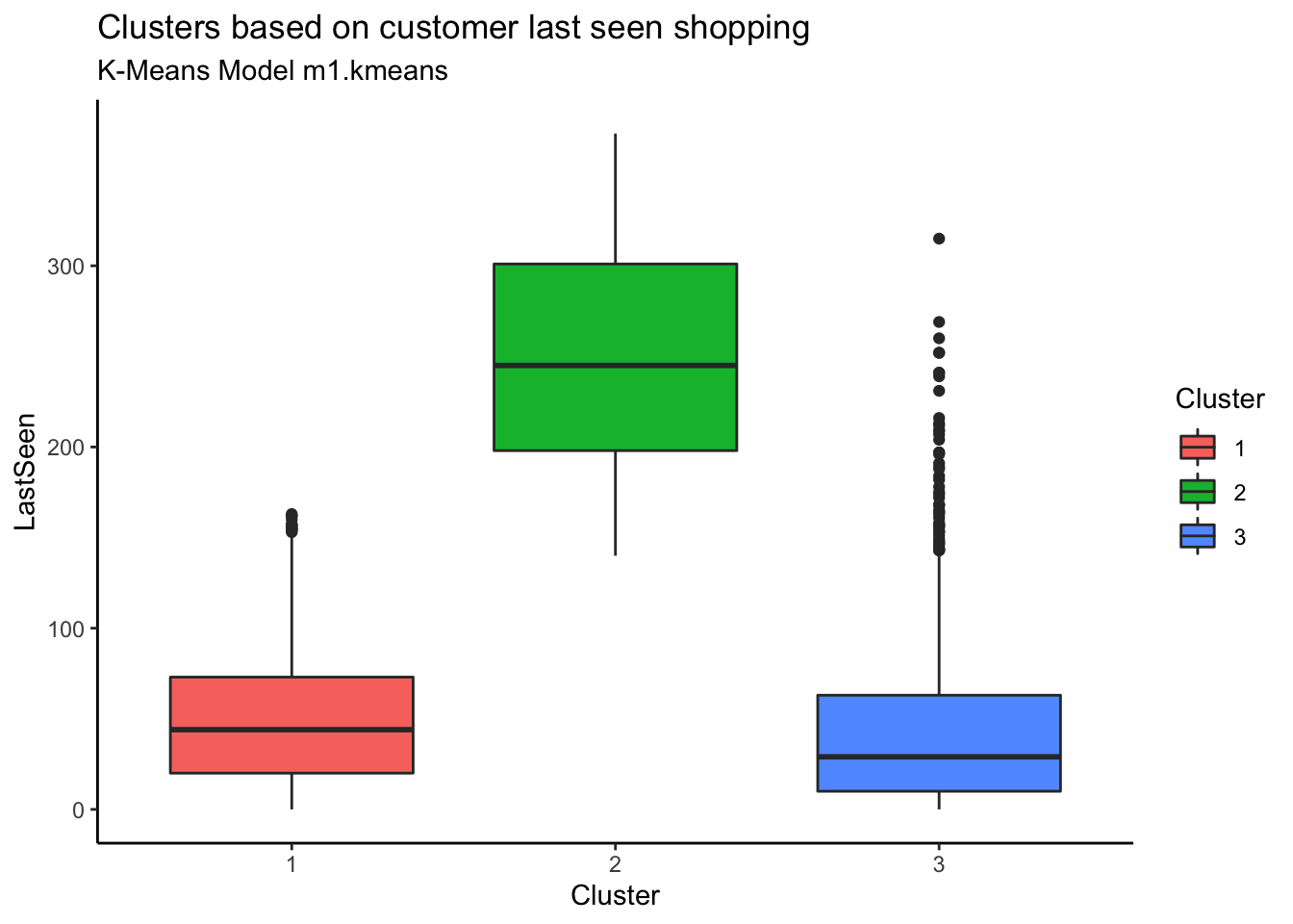
Customers in Cluster 2 have not been seen shopping recently. The most recently seen shoppers are in Cluster 3 and that also explains why they have spent more money and bought frequently

Why clustering isn’t (always) the answer?
Limitations
Challenging for large and highly dimensional datasets
- Difficult to visualize data
Developed in the 1960s
Before advent of the internet and “big data”
Not designed for datasets of such large scale
Convergence at Local Minimum/Local Optimum Solution
The algorithm is sensitive to:
Initial centroid value selection
Noise
Outliers
Clusters veer off and converge at local minimum rather than true global minimum
Shape of Data Clusters
The algorithm classifies n-hyperspherically shaped data well…
Less successful at classifying irregularly shaped clusters
How can we do it better?
Improvements
Researchers have developed many variations of the K-means algorithm to overcome limitations.
A “novel unsupervised k-means (U-k-means) clustering algorithm”
Created to overcome the challenge of selecting a K-value for very large datasets
No parameter initialization required
Built-in process determines K-value and performs K-means clustering using the concept of entropy
The K-value is initialized as the number of data points
Extra clusters are discarded until the “best” number of clusters is found
Method to determine K-value and detect and remove outliers and noise.
Regional density is calculated using a CLIQUE grid. Each dimension is divided into equal parts
The number of data points is calculated within each cell
Cells with counts above a defined threshold are defined as dense units. Adjacent dense units are connected to determine regional density
Noise in areas of low density is removed
Clustering by Fast Search and Find of Density Peaks. Method to approximate better initial cluster centroids.
Used in conjunction with CLIQUE
Local density of each point is calculated to determine optimum initial cluster centers
CLIQUE combined with CFSFDP can handle irregularly shaped clusters
Conclusion
K-Means clustering is a popular unsupervised learning algorithm
K-Means can be a great tool to achieve the segmentation of customers with speed and accuracy
K-Means is not always accurate and has some limitations
There are some improved algorithms that can help overcome these shortcomings.
Thank You!
